Simulate, Don’t Interpolate
Recovering continuous spatial dynamics from discrete, unpaired snapshots
Introduction
Many complex systems can only be understood through their change over time. Examples range from cell-fate decisions in biology[1] to chemical pattern formation[2] and grain growth in materials[3]. Modelling these systems requires understanding the processes that generate the observed states and govern their subsequent evolution. Yet complete trajectories are often difficult or impossible to observe. Destructive measurements, for example, provide detailed snapshots while preventing repeated observation of the same sample[4]. These observations provide a fragmented view of the system: they describe its marginal distributions at different times but do not directly reveal individual trajectories. Our aim is to learn a dynamical process from these unpaired snapshots, so that we can simulate how the system evolves and investigate its behaviour beyond the observed times or under local perturbations.
That is an ill-posed problem: distinct processes can produce the same distributions, so fitting the distributions alone cannot identify the dynamics that generated them[5]. Optimal transport[4], continuous flows[6] and stochastic bridges[7], flow matching[8] and stochastic interpolants[9], and recent multi-marginal and adversarially-learnt-interpolant variants[10][11][12][13] aim to reproduce the observed marginals, but the dynamics between them depend on modelling assumptions that the snapshots alone cannot determine. REGIS (REcovering Generative dynamics from Independent Snapshots) takes a different approach: it uses architectural constraints to narrow the space of rules that produce the unit system updates. These constraints come from our intuition about the modelled systems and, while being awkward to state about a probability path, they are often natural to state about an update rule. In this work, we focus on modelling spatial processes and therefore learn a rule that is local in space, Markovian and time-invariant, and which is applied iteratively to simulate the evolution of the system. We implement the rule as a neural cellular automaton[14][15] and train it adversarially[16] against the observed distributions, under the relativistic objective of R3GAN[17].
Below, we demonstrate that this approach can be applied to processes with very different dynamics: MNIST digits cycling through a sequence, a physical model of magnetism, and tissue regenerating after injury — learned from real spatial transcriptomics data. And because the rule is local and Markovian, the state can be edited part-way through the evolution, enabling in silico perturbations as experiments inside this framework without the need for any additional machinery.
Stable long-horizon dynamics
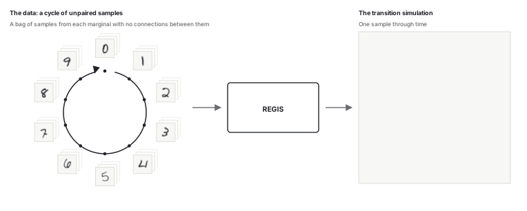
The handwritten digits in MNIST[18] have no natural time evolution, but we can define one: a cycle 0 → 1 → ⋯ → 9 → 0, learned as transitions from each digit to the next. The point of a cycle is that it never ends — once we have learned the rule, we can apply it sequentially and test the stability of the trajectories on ultra-long horizons. Starting from real test images we run up to 1000 consecutive transitions and measure the Fréchet distance[19] to real images in a frozen MNIST classifier’s feature space.
| Model | Parameters | Digit transitions completed | ||||
|---|---|---|---|---|---|---|
| 1 | 5 | 10 | 100 | 1000 | ||
| REGIS (ours) | 88 K | 37.228.9–54.4 | 28.121.9–44.4 | 45.728.8–49.9 | 20.819.1–25.3 | 21.418.9–24.7 |
| Non-local control Non-local control REGIS with a dilated update network[20] that can see the whole image in one update. It uses the same training procedure and a similar parameter count to isolate the effect of locality. | 83 K | 53.939.9–81.1 | 13155.7–270 | 208161–294 | 1,304†1,017–1,575 | 1,512†1,376–2,533 |
| MMSFM Multi-marginal stochastic flow matching A transport method that learns stochastic paths through several snapshot distributions using flow and score networks. Adapted here to overlapping triplets in the digit cycle. Lee, Moradijamei & Shakeri, 2025. [11] Multi-Marginal Stochastic Flow Matching for High-Dimensional Snapshot Data at Irregular Time Points | 18.6 M | 81.042.6–122 | 15986.7–215 | 46.626.9–66.6 | 262†160–1,272 | 34,928†5,498–64,357 |
| MMtSBM Multi-marginal temporal Schrödinger bridge matching Learns stochastic bridges connecting successive snapshot distributions, using forward and backward drift networks. Here, the transitions are arranged in a ten-digit loop. Gravier, Boyer & Genovesio, ICML 2026. [12] Multi-Marginal Temporal Schrödinger Bridge Matching from Unpaired Data | 3.6 M | 285195–429 | 303204–2,059 | 848184–6,176 | 1,596176–64,559 | 1,852†176–55,282 |
All models in the comparison perform well in the beginning; however, the gap increases over time and at the horizon of hundreds of digit transitions, REGIS is the only model that retains its initial quality. Models also take distinct approaches to the transition between digits, as illustrated in the video below - while REGIS gradually reshapes the stroke, reusing the present structures, other methods merely interpolate between digits or noise-denoise them.
Run the cycle yourself
The entire model has just 88 K parameters, making it suitable for in-browser local inference. Sample a real test digit or draw your own, press play, and leave it running! The simulation can run forever.
If you decide to draw your own digit, say a 3, note that it isn't trivial that the system automatically knows that it should produce a 4 next. No external classifier is involved, and all iterations are strictly local; therefore the model should first gather the information in a distributed fashion to understand what has been drawn. Such self-classifying behaviour has been reported before[21], but it's still fascinating to see it in a dynamic system.
Loading fetches the learned rule (368 KB) and 80 real MNIST test digits (80 KB), so you can run the cycle locally.
Start from
Run
Speed
Handwriting
The latent code is fixed during each run, but the updates are stochastic. Click above to change the code.
Data-efficient rule recovery and extrapolation
Cycling MNIST experiments show the model can hit a sequence of marginals, but this system lacks real underlying dynamics. To test whether REGIS can learn the process and not just copy the snapshots, we turn to the Ising model — a theoretical model of ferromagnetism that shows the behaviour of spins on a 2D lattice, evolving under Glauber dynamics[22]. We train REGIS on five marginal distributions, representing different timepoints in the coarsening process[23]: t ∈ {3, 10, 17, 300, 1000}.
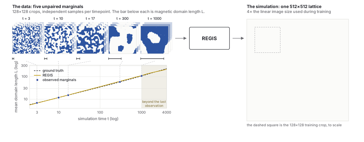
Since the true dynamics are known, we can evaluate REGIS on a much deeper level compared to the MNIST experiment. Beyond just matching the growth law, REGIS exhibits the following properties:
Extrapolation in time and spatial size. REGIS reproduces the ground-truth growth law up to t = 4000, four times the last observed time. The same rule also simulates 512 × 512 lattices after training on 128 × 128 crops, without retraining.
Data efficiency. REGIS learns the coarsening dynamics from as few as 50 unpaired snapshots. Even in this low data regime, the mean domain length remains close to ground truth, while the baseline diffusion model (DDPM)[24] exhibits a significant performance drop under low data budgets.
Recovery of the microscopic rule. We can inspect the learned rule by measuring the probability that a spin flips for each configuration of its neighbours. These probabilities match the true microscopic rule almost exactly; the largest deviations occur for flips that are very rare in the data.
Real world application recovers textbook biology
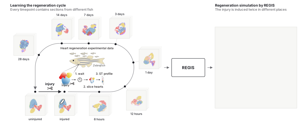
Many biological processes are inherently spatiotemporal: cell–cell interactions drive the formation and remodeling of tissue structure in development, regeneration, and diseases such as cancer. We therefore applied REGIS to a spatial atlas of adult zebrafish heart regeneration, which captures how the ventricle regrows after partial amputation [25]. Stereo-seq profiling of heart sections gives the spatial position of every annotated cell type in the uninjured heart and at seven timepoints after injury. The dataset is small — 4–6 hearts per timepoint, three sections per heart — and presents the typical obstacles of biological data: measurement is destructive, so paired observations are impossible, and heart shape varies considerably between individuals. The trained model simulates the otherwise unobservable trajectory of an individual heart's response to an in silico injury.
Interactive heart regeneration simulator
As in the MNIST experiment, the model is small enough to run locally in your browser. Click on the blue region to injure the heart and watch it regenerate. The injury triggers a cascade in which border-zone cardiomyocytes (Bzm) activate, dedifferentiate, proliferate, and redifferentiate, accompanied by the appearance of stromal cells that help regulate regeneration. None of these steps were ever observed in the heart you are simulating: every change follows solely from the learned local, time-invariant update rule.
Loading the heart simulation…
Or draw your own cut. Drag on the blue ventricle, then press Play.
Cell activity and colour key
The plots track cell density as the heart regenerates. Each line uses the cell type’s colour in the key below.
Colour shows the dominant cell type; opacity reflects tissue density. Border-zone myocardium (BZm) states are highlighted when they exceed their 99.7th-percentile thresholds.
The training data contain cuts to the ventricular apex. Cuts to the yellow bulbus arteriosus or red atrium fall outside those observations.
Does it reflect known biology?
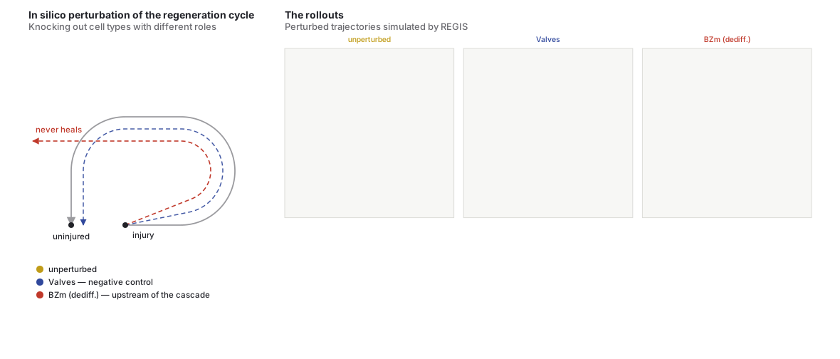
Complete experimental trajectories cannot be observed, so we cannot compare them with the simulated ones directly. We can, however, test whether the model reproduces known biological relationships. Heart regeneration involves border-zone cardiomyocytes (Bzm), the heart muscle cells near the injury, together with macrophages, pro-regenerative fibroblasts, and epicardial cells. The cardiomyocytes pass through activation, dedifferentiation, proliferation, and redifferentiation — the sequence that defines the regeneration cascade [25]. If the learned dynamics reflect this sequence, suppressing one state should disrupt the states downstream of it, which gives a falsifiable prediction.
We test this prediction with in silico knockouts, setting the abundance of a selected cell population to zero after every simulation update. We then compare the cell composition at 28 days after injury with that of the unperturbed simulation and measure how the knockout changes the cardiomyocyte response. Valve cells serve as a negative control, since they are not involved in regeneration.
Knocking out regeneration-associated populations stops the system before the end of the cascade, leaving the simulated heart far from the healed state. Knocking out valve cells, in contrast, leaves simulated healing intact. The model was never trained on knockout experiments: these responses emerge from a rule learned only from unpaired snapshots.
Conclusion
Learning a local, time-invariant rule lets us turn unpaired snapshots into a process we can simulate and perturb. In the examples above, this was enough to sustain long trajectories, extrapolate beyond the training data, and recover meaningful dependencies between cell states. As spatial technologies become widely available, we hope this approach will help us study processes whose individual trajectories cannot be observed.
Bonus: REGIS on non-regular grids
Replacing the 2D convolution in the perception layer with a graph convolution lets the same kind of rule run on arbitrary arrangements of cells. As a proof of concept, we train the cycling-MNIST task on digits placed on random packings of 200 discs. Neighbouring cells are connected by a Delaunay triangulation, and the Sobel filters are replaced by a least-squares estimate of each channel’s gradient over a cell’s neighbours (this becomes the vanilla NCA’s Sobel filter on a square lattice). Everything else in the generator is the same.
Once trained, the rule is not tied to the grids it was trained on: at inference it carries over to regular lattices it has never seen, and even to grids whose nodes are moving.
References
- p53 Dynamics Control Cell Fate. Science 336, 1440–1444, 2012. doi
- Transition from a Uniform State to Hexagonal and Striped Turing Patterns. Nature 352, 610–612, 1991. doi
- Grain Growth in Four Dimensions: A Comparison between Simulation and Experiment. Acta Materialia 78, 125–134, 2014. doi
- Optimal-Transport Analysis of Single-Cell Gene Expression Identifies Developmental Trajectories in Reprogramming. Cell 176, 928–943.e22, 2019. doi
- Fundamental Limits on Dynamic Inference from Single-Cell Snapshots. PNAS 115, E2467–E2476, 2018. doi
- TrajectoryNet: A Dynamic Optimal Transport Network for Modeling Cellular Dynamics. ICML, 2020. pmlr
- Simulation-Free Schrödinger Bridges via Score and Flow Matching. AISTATS, 2024. pmlr
- Flow Matching for Generative Modeling. ICLR, 2023. openreview
- Stochastic Interpolants: A Unifying Framework for Flows and Diffusions. JMLR 26(209), 1–80, 2025. jmlr
- Modeling Complex System Dynamics with Flow Matching across Time and Conditions. ICLR, 2025. iclr
- Multi-Marginal Stochastic Flow Matching for High-Dimensional Snapshot Data at Irregular Time Points. 2025. arXiv:2508.04351
- Multi-Marginal Temporal Schrödinger Bridge Matching from Unpaired Data. ICML, 2026. arXiv:2510.01894
- Multi-Marginal Flow Matching with Adversarially Learnt Interpolants. ICLR, 2026. arXiv:2510.01159
- Growing Neural Cellular Automata. Distill, 2020. distill.pub
- Learning Spatio-Temporal Patterns with Neural Cellular Automata. PLOS Comput. Biol. 20, e1011589, 2024. doi
- Generative Adversarial Nets. NeurIPS, 2014. neurips
- The GAN is Dead; Long Live the GAN! A Modern GAN Baseline. NeurIPS, 2024. neurips
- Gradient-Based Learning Applied to Document Recognition. Proc. IEEE 86, 2278–2324, 1998. doi
- GANs Trained by a Two Time-Scale Update Rule Converge to a Local Nash Equilibrium. NeurIPS, 2017. neurips
- Multi-Scale Context Aggregation by Dilated Convolutions. ICLR, 2016. arXiv:1511.07122
- Self-classifying MNIST Digits. Distill, 2020. distill.pub
- Time-Dependent Statistics of the Ising Model. J. Math. Phys. 4, 294–307, 1963. doi
- Theory of Phase-Ordering Kinetics. Advances in Physics 43, 357–459, 1994. doi
- Denoising Diffusion Probabilistic Models. NeurIPS, 2020. neurips
- An Organ-Wide Spatiotemporal Transcriptomic and Cellular Atlas of the Regenerating Zebrafish Heart. Nature Communications 16, 3716, 2025. doi